Kreechers: Cellular Automata Playground

It's life ^*John, but not as we know it

"So," you may be asking, "what's all this then, just another ver­sion of ^*John Conway's Life?". An under­stand­able ques­tion, but the answer is no, it's actually something quite different and new, and also sort of yes, in that it's all about ones and zeros in a binary 2D world, so it may remind you of the original Life program from 1970.

To under­stand the diff­erence between Kreechers and the Game of Life, and to explain what's going on, let's quickly recap on how the original program works. The idea is that the Game of Life takes place on a two-dimen­sional world, much like graph paper. In fact, it used to be played on graph paper before pro­grams were written to run it.

There are two simple rules to follow, from which a tremen­dous number of unex­pected results can occur. These rules are:

1. If a square is empty but exactly three of its neigh­bors (on the edges and diag­onals) are full (see Figure 1), then the square is filled (emul­ating giving birth).


2. If a square is filled, but there are either fewer than two or more than three filled neigh­boring squares (as in Figure 2) then the square becomes empty, emu­lating death

There is, as it happens, a sort of third rule, which isn't really a rule because it simply states that if none of the above is true then no change occurs to the square.

Each square in turn on the graph paper (or in an array in a computer, which can be as large as you like) is then proces­sed in this way until a sheet is comp­leted. Then the whole process starts all over again at the first square, and contin­ues ad-infin­itum.

"Simple enough," you might think, if you've never come across the game before, but the results of care­fully placing a few init­ially filled squares can be stagger­ingly complex. In fact, it has been proven that The Game of Life is 100% Turing complete, which means that it has the capa­bility to perform any compu­tations that a regular computer can, and there are even config­urations of the game which recurs­ively simulate the game itself, thus neatly proving the point!

You can also play the Game of Life in Kreechers (and in color too!) by pres­sing the button in the panel. After a while you will notice how many config­urat­ions wind up with a stable pattern, and others even result in total wipeout. With care­fully placed initial cells, how­ever, you can achieve quite inter­esting results.

Figure 3

More than that, instead of the standard rules of Life, you can try any of the 256² other rules too, many of which create stunning mosaics, crystalline shapes and colonies, as shown in Figure 3.

Inci­den­tally, the colors (which you don't often see in the Game of Life) were chosen to slowly cycle according to how old the particles are, star­ting over again if a par­ticle dies and is rep­laced by a new one.

How Kreechers Works

Under the hood

The main thing about Kreechers is that there is no birth or death, and there­fore the total number of filled locat­ions always remains the same, unless you add or remove any using the mouse or buttons prov­ided. Instead, movement and change occur by swapping the contents of locat­ions accor­ding to sets of rules.

So let's start off with the same piece of graph paper used for Life, but then choose any sized matrix from 1×1 to 9×9. The mathe­matics allows for any sized matrix, but for reasons of practi­cality and the speed of current com­puters, 9 has been chosen as the maximum for this program.

Now, pass the matrix across the graph paper one positon at a time and apply a set of swap rules based on whether or not a cell under the matrix is filled. Let's take the case of using a 2×2 matrix to process the graph paper. As shown in Figure 4, there are four locations to examine. For each cell in the matrix a swap rule is applied if the square under the cell is filled. In the case of this figure, only the bottom-left location is filled.

In a 2×2 matrix there are 7 possible swap rules that can be applied, which are:

1. Don't do anything
2. Swap Top-Left and Top-Right
3. Swap Top-Left and Bottom Left
4. Swap Top-Left and Bottom-Right
5. Swap Top-Right and Bottom-Left
6. Swap Top-Right and Bottom-Right
7. Swap Bottom-Left and Bottom-Right

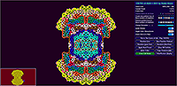
Looking at the program running at the top of this page, you can see such a 2×2 matrix at the top-left of the window, and in it there are some filled and empty squares. The filled squares re­pre­sent the swaps to be made if a cell under one of the four posit­ions is filled. If only a single cell is shown in the matrix then the location is swapped with itself, which means nothing happens and this is how swap rule 1, "Don't do anything", works.

So, in the case of the default 2×2 rules, when this page first loads the rule matrix looks like Figure 5. Taking the data from Figure 4 of just the single bottom-left location being filled, we then look at the rule matrix and see that the bottom-left rule is to swap the top-left and bottom-right locations.

In this part­icular case, however, the swap will have no effect because the top-left and bottom-right loca­tions are both the same (empty), and so there will be no noticable change (in fact the program knows this and just does nothing). However, should Figure 5 contain locations in the config­uration of Figure 6, in which the top-left location is also filled, then the swap rule would end up making Figure 6 look like Figure 7, once the swap has been per­formed.

So, unlike Life, in which the two rules are fixed, in Kreechers the rules depend on which locations are already filled and, by swapping them around, the rules to be ap­plied cons­tantly change. More than that, you can choose between the seven diff­erent rules for each cell position in a 2×2 matrix, giving you 7×7×7×7 (7⁴), or a total of 2,401 diff­erent possible combin­ations of rules. So already there are over a couple of thou­sand vari­ations of the 2×2 version of Kreechers, which makes for some very inter­esting and varied results.

But this is just the beginning, because you can extend the size of the rule matrix in a multitude of diff­erent ways to get even more results and, if you choose a 9×9 matrix, for example, there are more than 10²⁸⁴ possible combin­ations – several orders of magitude greater than the total number of atoms in the Universe!

But wait, there's more!

Not only, but also...

With matrixes larger than 2×2 the rules allow for swapping any of the cells under the matrix (not just a 2×2 section), even up to 81 of them under a 9×9 matrix. There is, how­ever, an issue when the matrix gets large, in that due to the enor­mous num­ber of pos­sible rule sets, huge num­bers of them are (to us) quite un­in­ter­est­ing and res­emble chaos. They are not cha­otic, in fact, but are just too comp­lex for us to vis­ually take in.

So, to help us mortal humans under­stand the larger matrix­es, I have added a switch with which you can limit the action of each of the rules in a matrix to just those swaps sup­ported in a basic 2×2 matrix, as in Figure 8, where you can see the squares repre­senting the locations under the matrix where the rules will be applied are shown in red.

These rules are applied to the four cells nearest to the center (of course it could have been any set of four cells, so I just opted for the middle), underneath the matrix. Even then, with a 9×9 matrix you still have more than 10⁶⁸ pos­sible comb­ina­tions (per­haps just shy of the number of atoms in the Uni­verse), but many, many more of them show some sort of pattern or be­hav­iour we can under­stand.

Figure 9

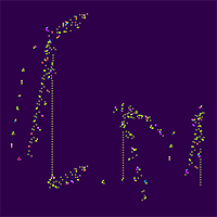
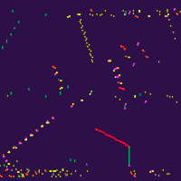
To get started with this program, perhaps you may wish to click the [Apply Next Preset] button (or press 'A') now and then, and watch the results of simply writing the word 'Kreechers' into the world's empty loca­tions. Note that the presets load into the current zoom level, so you will see dif­ferent results depen­ding on how far you are zoomed in or out. You will soon see many types of gliders and flyers (as in Figure 9), complex line crawlers (see Figure 10), and much more.

For example, try zooming in and out, as well as changing the matrix sizes, and turn on the mutation feature to auto­matic­ally make one rule change in a rule set every 15 seconds (be patient though, some changes are very subtle). When mutation is on, the top-left matrix will high­light the most recent rule change.

You can directly change single rules in a matrix by click­ing (and double-clicking) the cells to be changed, and you can also draw on the world with the mouse to fill empty loca­tions with par­ticles. This can be easier to do if you pause ani­mation first. For even better preci­sion, draw in Edit Mode, which pauses animation for you and also stabi­lises the panning window (unless [Shift] is held down, in which case you can pan to wherever you wish to edit). Right-clicking on any of the draw func­tions erases instead of drawing. Pausing and stepping will reveal much about the current rule set.

Figure 10

The colors shown are assig­ned accor­ding to how many times a parti­ has had its loca­tion swapped during each frame scan. Interes­tingly this displays a lot of pat­ter­ning and also regu­larity too. Looking at even the very first preset using this colori­zation, I get the feeling that very many matrix sizes and rule sets are Turing complete, and it should be possible to create complex and fanci­ful compu­tations (starting with simple logic gates and moving up) much more quickly and easily than with Life. To this end I will shortly release a Pattern Editor - watch this space.

If you create anything with this or develop it further, please accredit my work when you do so, thanks! And feel free to brainstorm with me at robin@­robinnixon­.com. Here is the Github Repository.